Evaluation#
The Evaluation class is the actual interface for the user with the
functionalities of the pyEvalData package. It provides access to the raw
data via the Source object, given on initialization.
The main features of the Evaluation class are the definition of counter
aliases as well as new counters by simple algebraic expressions.
At the same time pre- and post-filters can be applied to the raw and
evaluated data, respectively.
Much efforts have been put into the binning, averaging, and error calculation
of the raw data.
In addition to the evaluation of a list of scans or scan sequence of one or
multiple scans in dependence of an external paramter, the Evaluation class
also provides high-level helper functions for plotting and fitting the
according results.
Setup#
Here we do the necessary import for this example
%load_ext autoreload
%autoreload 2

import matplotlib.pyplot as plt
import numpy as np

import pyEvalData as ped
# import lmfit for fitting
import lmfit as lf
# import some usefull fit functions
import ultrafastFitFunctions as ufff
# define the path for the example data
example_data_path = '../../../example_data/'
Source#
Here we iitialize the Source for the current evaluation. It is based on raw
data in a SPEC file which was generated by
the open-source software Sardana.
spec = ped.io.Spec(file_name='sardana_spec.spec',
                   file_path=example_data_path,
                   use_nexus=True,
                   force_overwrite=False,
                   update_before_read=False,
                   read_and_forget=True)
pyEvalData.io.source - INFO: Update source
pyEvalData.io.source - INFO: parse_raw
pyEvalData.io.source - INFO: Create spec_file from xrayutilities
XU.io.SPECFile.Update: reparsing file for new scans ...
pyEvalData.io.source - INFO: save_all_scans_to_nexus
pyEvalData.io.source - INFO: read_raw_scan_data for scan #1
XU.io.SPECScan.ReadData: scan_1: 291 27 27
pyEvalData.io.source - INFO: save_scan_to_nexus for scan #1
pyEvalData.io.source - INFO: read_raw_scan_data for scan #2
XU.io.SPECScan.ReadData: scan_2: 291 27 27
pyEvalData.io.source - INFO: save_scan_to_nexus for scan #2
pyEvalData.io.source - INFO: read_raw_scan_data for scan #3
XU.io.SPECScan.ReadData: scan_3: 291 27 27
pyEvalData.io.source - INFO: save_scan_to_nexus for scan #3
pyEvalData.io.source - INFO: read_raw_scan_data for scan #4
XU.io.SPECScan.ReadData: scan_4: 291 27 27
pyEvalData.io.source - INFO: save_scan_to_nexus for scan #4
pyEvalData.io.source - INFO: read_raw_scan_data for scan #5
XU.io.SPECScan.ReadData: scan_5: 291 27 27
pyEvalData.io.source - INFO: save_scan_to_nexus for scan #5
pyEvalData.io.source - INFO: read_raw_scan_data for scan #6
XU.io.SPECScan.ReadData: scan_6: 291 27 27
pyEvalData.io.source - INFO: save_scan_to_nexus for scan #6
The Evaluation class#
For the most basic example we just have to provide a Source on initialization:
ev = ped.Evaluation(spec)
Now it is possible to check the available attributes of the Evaluation
object, which will be explained step-by-step in the upcominng sections.
print(ev.__doc__)
Evaluation

    Main class for evaluating data.
    The raw data is accessed via a ``Source`` object.
    The evaluation allows to bin data, calculate errors and propagate them.
    There is also an interface to ``lmfit`` for easy batch-fitting.

    Args:
        source (Source): raw data source.

    Attributes:
        log (logging.logger): logger instance from logging.
        clist (list[str]): list of counter names to evaluate.
        cdef (dict{str:str}): dict of predefined counter names and
            definitions.
        xcol (str): counter or motor for x-axis.
        t0 (float): approx. time zero for delay scans to determine the
            unpumped region of the data for normalization.
        custom_counters (list[str]): list of custom counters - default is []
        math_keys (list[str]): list of keywords which are evaluated as numpy functions
        statistic_type (str): 'gauss' for normal averaging, 'poisson' for counting statistics
        propagate_errors (bool): propagate errors for dpendent counters.
Most of the attributes of the Evaluation class are well explained in the docstring above
and described in more details below.
The custom_counters might be soon depricated.
The t0 attribute is used for easy normalization to 1 by
dividing the data by the mean of all values which are xcol < t0.
This is typically useful for time-resolved delay scans but might be renamed
for a more general approach in the future.
The statistics_type attribute allows to switch between gaussian statistics,
which calculates the error from the standard derivation, and poisson statistics,
whichs calculates the error from $1/\sqrt N$ with $N$ being the total number of
photons in the according bin.
Simple plot example#
To plot data, the Evlauation objects does only need to know the xcol as
horizontal axis as well a list of counters to plot, which is called clist.
First we can check the available scan numbers in the source:
spec.get_all_scan_numbers()
[1, 2, 3, 4, 5, 6]
Now we can check for the available data for a specific scan
spec.scan1.data.dtype.names
('Diff',
 'DiffM',
 'Pt_No',
 'Pumped',
 'PumpedErr',
 'PumpedErrM',
 'PumpedM',
 'Rel',
 'RelM',
 'Unpumped',
 'UnpumpedErr',
 'UnpumpedErrM',
 'UnpumpedM',
 'chirp',
 'delay',
 'dt',
 'duration',
 'durationM',
 'envHumid',
 'envTemp',
 'freqTriggers',
 'magneticfield',
 'numTriggers',
 'numTriggersM',
 'thorlabsPM',
 'thorlabsPPM',
 'thorlabsPPMonitor')
So let’s try to plot the counters Pumped and Unpumped vs the motor delay for scan #1:
ev.xcol = 'delay'
ev.clist = ['Pumped', 'Unpumped']

plt.figure()
ev.plot_scans([1])
plt.xlim(-10, 50)
plt.xlabel('delay (ps)')
plt.show()
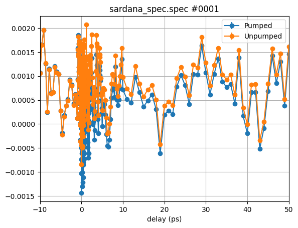
Algebraic expressions#
For now, we only see a lot of noise. So let’s work a bit further on the data we
plot. The experiment was an ultrafast MOKE
measurement, which followed the polarization rotation of the probe pulse after
a certain delay in respect to the pump pulse. Typically, this magnetic contrast
is improved by subtracting the measured signal for two opposite magnetization
directions of the sample, as the MOKE effect depends on the sample’s magnetization.
In our example, we have two additional counters available, which contain the
data for negative magnetic fields (M - minus): PumpedM and UnpumpedM
While the two former counters were acquired for positive fields.
Let’s plot the difference signal for the pumped and unpumped signals:
ev.xcol = 'delay'
ev.clist = ['Pumped-PumpedM', 'Unpumped-UnpumpedM']

plt.figure()
ev.plot_scans([1])
plt.xlim(-10, 50)
plt.xlabel('delay (ps)')
plt.show()
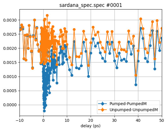
The new plot shows already much more dynamisc in the pumped vs. the unpumped signal. However, we can still improve that, by normalizing one by the other:
ev.xcol = 'delay'
ev.clist = ['(Pumped-PumpedM)/(Unpumped-UnpumpedM)']

plt.figure()
ev.plot_scans([1])
plt.xlim(-10, 50)
plt.xlabel('delay (ps)')
plt.show()
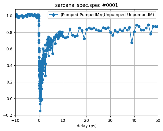
This does look much better but we lost the absolute value of the contrast. Let’s simply multiply the trace with the average of the unpumped magnetic contrast:
ev.xcol = 'delay'
ev.clist = ['(Pumped-PumpedM)/(Unpumped-UnpumpedM)*mean(Unpumped-UnpumpedM)']

plt.figure()
ev.plot_scans([1])
plt.xlim(-10, 50)
plt.xlabel('delay (ps)')
plt.show()
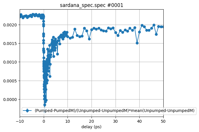
So besides simple operations such as +. -. *, / we can also use some basic
numpy functionalities. You can check the available functions by inspection
of the attribute math_keys:
ev.math_keys
['mean',
 'sum',
 'diff',
 'max',
 'min',
 'round',
 'abs',
 'sin',
 'cos',
 'tan',
 'arcsin',
 'arccos',
 'arctan',
 'pi',
 'exp',
 'log',
 'log10',
 'sqrt',
 'sign']
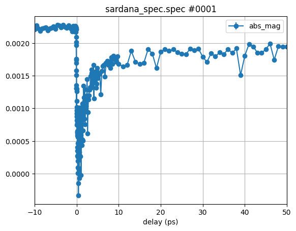
But of course our current counter name is rather bulky. So lets define some
aliases using the attribute cdef:
ev.cdef['pumped_mag'] = 'Pumped-PumpedM'
ev.cdef['unpumped_mag'] = 'Unpumped-UnpumpedM'
ev.cdef['rel_mag'] = 'pumped_mag/unpumped_mag'
ev.cdef['abs_mag'] = 'pumped_mag/unpumped_mag*mean(unpumped_mag)'
ev.xcol = 'delay'
ev.clist = ['abs_mag']

plt.figure()
ev.plot_scans([1])
plt.xlim(-10, 50)
plt.xlabel('delay (ps)')
plt.show()
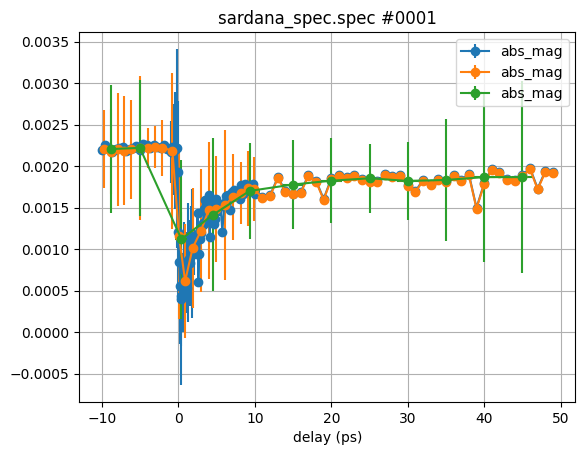
Binning#
In many situations it is desireable to reduce the data density or to plot the
data on a new grid. This can be easily achieved by the xgrid keyword of the
plot_scans method.
Here we plot the same data as before on a three reduced grids with 0.1, 1, and
5 ps step width. Please note that the errorbars appear due to the averaging of
multiple point in the bins of the grid. The errorbars are vertical and horizontal.
We can also skip the xlim setting here, as our grid is in the same range as
before.
ev.xcol = 'delay'
ev.clist = ['abs_mag']

plt.figure()
ev.plot_scans([1], xgrid=np.r_[-10:50:0.1])
ev.plot_scans([1], xgrid=np.r_[-10:50:1])
ev.plot_scans([1], xgrid=np.r_[-10:50:5])
plt.xlabel('delay (ps)')
plt.show()
Averaging & error propagation#
In order to improve statistics even further, scans are often repeated an averaged. This was also done for this experimental example and all scans #1-6 were done with the same settings.
We can simply average them by providing all scans of interest to the plot_scans
method:
ev.xcol = 'delay'
ev.clist = ['abs_mag']

plt.figure()
ev.plot_scans([1, 2, 3, 4, 5, 6], xgrid=np.r_[-10:50:0.1])
plt.xlabel('delay (ps)')
plt.show()
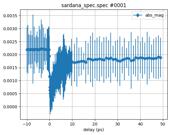
Hm, somehow this did not really did the job, right? Altough the scattering of the circle symbols has decreased, the errorbars are much large as for the single scan before.
Let’s check the individual scans to see what happened:
ev.xcol = 'delay'
ev.clist = ['abs_mag']

plt.figure()
ev.plot_scans([1], xgrid=np.r_[-10:50:0.1])
ev.plot_scans([2], xgrid=np.r_[-10:50:0.1])
ev.plot_scans([3], xgrid=np.r_[-10:50:0.1])
ev.plot_scans([4], xgrid=np.r_[-10:50:0.1])
ev.plot_scans([5], xgrid=np.r_[-10:50:0.1])
ev.plot_scans([6], xgrid=np.r_[-10:50:0.1])
plt.xlabel('delay (ps)')
plt.show()
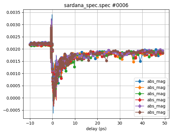
Individually all scans look very much the same, with very small errorbars. So why do we get so large errorbars when we average them?
Let’s go one more step back and plot the Unpumped signal for all scans with a
large grid of 5 ps for clarity:
ev.xcol = 'delay'
ev.clist = ['Unpumped']

plt.figure()
ev.plot_scans([1], xgrid=np.r_[-10:50:5])
ev.plot_scans([2], xgrid=np.r_[-10:50:5])
ev.plot_scans([3], xgrid=np.r_[-10:50:5])
ev.plot_scans([4], xgrid=np.r_[-10:50:5])
ev.plot_scans([5], xgrid=np.r_[-10:50:5])
ev.plot_scans([6], xgrid=np.r_[-10:50:5])
plt.xlabel('delay (ps)')
plt.show()
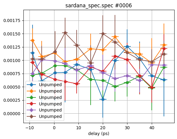
We can observe a significant drift of the raw data which results in deviations that are not statistically distributed anymore.
This essentially means, that it makes a difference if we
evaluate the expression
abs_magfor every scan individually and eventually average the resulting tracesfirst average the raw data (
Pumped, PumpedM, Unpumped, UnpumpedM) and then calculate final trace forabs_magusing the averaged raw data. In the later case we need to carry out a proper error propagation to determine the errors forabs_mag.
The Evaluation class allows to switch between both cases by the attribute flag
propagate_errors which is True by default and handles the error propagation
automatically using the uncertainties package.
For our last example we were follwoing option 2. as described above.
Accoridngly, rather large errors from the drifiting of the raw signals were propagated.
Now lets compare to option 1. without error propagation:
ev.xcol = 'delay'
ev.clist = ['abs_mag']

plt.figure()
ev.propagate_errors = True
ev.plot_scans([1, 2, 3, 4, 5, 6], xgrid=np.r_[-10:50:0.1])

ev.propagate_errors = False
ev.plot_scans([1, 2, 3, 4, 5, 6], xgrid=np.r_[-10:50:0.1])
plt.xlabel('delay (ps)')
plt.legend(['error propagation', 'no error propagation'])
plt.show()
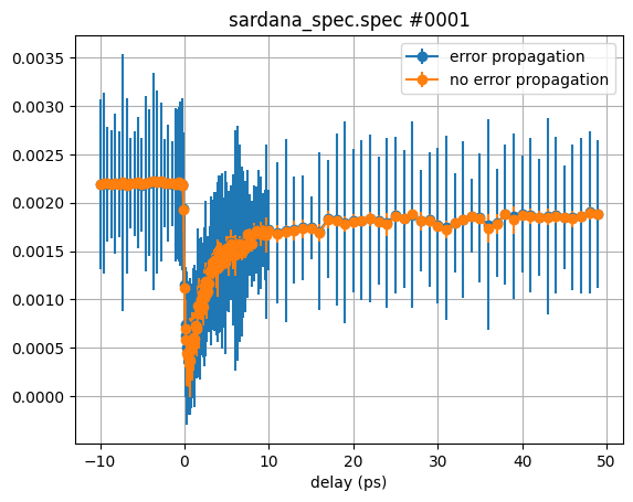
The application of the both options strongly depends on the type of noise and drifts of the acquired data.
plot_scans() options#
Let’s check all arguments of the plot_scans() method by simply calling:
help(ev.plot_scans)
Help on method plot_scans in module pyEvalData.evaluation:

plot_scans(scan_list, ylims=[], xlims=[], fig_size=[], xgrid=[], yerr='std', xerr='std', norm2one=False, binning=True, label_text='', title_text='', skip_plot=False, grid_on=True, ytext='', xtext='', fmt='-o') method of pyEvalData.evaluation.Evaluation instance
    Plot a list of scans from the spec file.
    Various plot parameters are provided.
    The plotted data are returned.

    Args:
        scan_list (List[int])        : List of scan numbers.
        ylims (Optional[ndarray])   : ylim for the plot.
        xlims (Optional[ndarray])   : xlim for the plot.
        fig_size (Optional[ndarray]) : Figure size of the figure.
        xgrid (Optional[ndarray])   : Grid to bin the data to -
                                      default in empty so use the
                                      x-axis of the first scan.
        yerr (Optional[ndarray])    : Type of the errors in y: [err, std, none]
                                      default is 'std'.
        xerr (Optional[ndarray])    : Type of the errors in x: [err, std, none]
                                      default is 'std'.
        norm2one (Optional[bool])   : Norm transient data to 1 for t < t0
                                      default is False.
        label_text (Optional[str])   : Label of the plot - default is none.
        title_text (Optional[str])   : Title of the figure - default is none.
        skip_plot (Optional[bool])   : Skip plotting, just return data
                                      default is False.
        grid_on (Optional[bool])     : Add grid to plot - default is True.
        ytext (Optional[str])       : y-Label of the plot - defaults is none.
        xtext (Optional[str])       : x-Label of the plot - defaults is none.
        fmt (Optional[str])         : format string of the plot - defaults is -o.

    Returns:
        y2plot (OrderedDict)    : y-data which was plotted.
        x2plot (ndarray)        : x-data which was plotted.
        yerr2plot (OrderedDict) : y-error which was plotted.
        xerr2plot (ndarray)     : x-error which was plotted.
        name (str)              : Name of the data set.
Most of the above arguments are plotting options and will be changed/simplified
in a future release.
The xerr and yerr arguments allow to change the type of errorbars in x and y
direction between standard error, standard derivation and no error.
The norm2one flag allows to normalize the data to 1 for all data which is before
Evaluation.t0 on the xcol.
The skip_plot option disables plotting at all and can be handy if only access to
the return values is desired.
The returned data contains the xcol and according error as ndarray named x2plot
and xerr2plot, while the according counters and errors from the clist are given
as OrderedDicts y2plot and yerr2plot. The keys of these dictionaries
correspond to the elements in the clist.
Scan sequences#
Experimentally it is common to repeat similar scans while varying an external parameter,
such as the sample environment (temperature, external fields, etc.).
For this common task, the Evaluation class provides a method named
plot_scan_sequence() which wraps around the plot_scans() method.
First, we have to define the scan_sequence as a nested list to be correctly parsed
by the plot_scan_sequence() method.
For that, we use the day time of the scans as an external parameter.
We can access such meta information directly from the Source object as follows:
print(spec.scan1.time)
print(spec.scan2.time)
print(spec.scan3.time)
print(spec.scan4.time)
print(spec.scan5.time)
print(spec.scan6.time)
21:28:49
00:05:09
02:27:56
05:03:44
07:39:54
10:16:11
Now we create the scan_sequence as a list, which contains one or multiple
entries. Each entry can be a list or tuple which contains two elements:
The scan list containing one or multiple scan numbers, and a string or number
describing the external parameter.
scan_sequence = [
    # ([scan numbers], parameter)
    ([1], spec.scan1.time),  # first entry
    ([2], spec.scan2.time),
    ([3], spec.scan3.time),
    ([4], spec.scan4.time),
    ([5], spec.scan5.time),
    ([6], spec.scan6.time),  # last entry
]
The minimum example below does not differ too much from plotting all six scans
manually by the plot_scans() method:
plt.figure()
ev.plot_scan_sequence(scan_sequence)
plt.show()
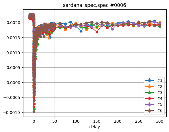
Obviously, the legend did not take the scan time into account. Let’s check the documentation for some details:
help(ev.plot_scan_sequence)
Help on method plot_scan_sequence in module pyEvalData.evaluation:

plot_scan_sequence(scan_sequence, ylims=[], xlims=[], fig_size=[], xgrid=[], yerr='std', xerr='std', norm2one=False, binning=True, sequence_type='', label_text='', title_text='', skip_plot=False, grid_on=True, ytext='', xtext='', fmt='-o') method of pyEvalData.evaluation.Evaluation instance
    Plot a list of scans from the spec file.
    Various plot parameters are provided.
    The plotted data are returned.

    Args:
        scan_sequence (List[
            List/Tuple[List[int],
            int/str]])              : Sequence of scan lists and parameters.
        ylims (Optional[ndarray])   : ylim for the plot.
        xlims (Optional[ndarray])   : xlim for the plot.
        fig_size (Optional[ndarray]) : Figure size of the figure.
        xgrid (Optional[ndarray])   : Grid to bin the data to -
                                      default in empty so use the
                                      x-axis of the first scan.
        yerr (Optional[ndarray])    : Type of the errors in y: [err, std, none]
                                      default is 'std'.
        xerr (Optional[ndarray])    : Type of the errors in x: [err, std, none]
                                      default is 'std'.
        norm2one (Optional[bool])   : Norm transient data to 1 for t < t0
                                      default is False.
        sequence_type (Optional[str]): Type of the sequence: [fluence, delay,
                                      energy, theta, position, voltage, none,
                                      text] - default is enumeration.
        label_text (Optional[str])   : Label of the plot - default is none.
        title_text (Optional[str])   : Title of the figure - default is none.
        skip_plot (Optional[bool])   : Skip plotting, just return data
                                      default is False.
        grid_on (Optional[bool])     : Add grid to plot - default is True.
        ytext (Optional[str])       : y-Label of the plot - defaults is none.
        xtext (Optional[str])       : x-Label of the plot - defaults is none.
        fmt (Optional[str])         : format string of the plot - defaults is -o.

    Returns:
        sequence_data (OrderedDict) : Dictionary of the averaged scan data.
        parameters (List[str, float]) : Parameters of the sequence.
        names (List[str])          : List of names of each data set.
        label_texts (List[str])     : List of labels for each data set.
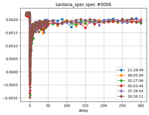
In the docstring we can find many arguments already known from the plot_scans()
method. In order to fix the legend labels we need to tell the method about the
sequence_type as an argument. Otherwise it will enumerate the scans by default.
In our case we provided a text type label:
plt.figure()
sequence_data, parameters, names, label_texts = \
    ev.plot_scan_sequence(scan_sequence, sequence_type='text')
plt.show()
In the example above we also catched the return values. Here the parameters
correspond exactly to the data we provided in the scan_sequence while the
label_texts are the formatted string as written in the legend.
The names correspond to the auto-generated name of each scan as given by
the plot_scans() method.
The actual sequence_data is again an OrderedDict where the keys are given
by the strings in the xcol and clist attributes of the Evaluation object.
Each value for a given key is a list of ndarrays that hold the data for
every parameter.
print(sequence_data.keys())
odict_keys(['delay', 'delayErr', 'abs_mag', 'abs_magErr'])
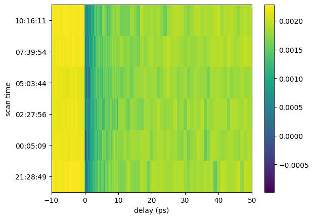
Let’s make an 2D plot from the scan_sequence:
x = sequence_data['delay'][0]
y = np.arange(6)
z = sequence_data['abs_mag']

plt.figure()
plt.pcolormesh(x, y, z, shading='auto')
plt.xlim(-10, 50)
plt.xlabel('delay (ps)')
plt.yticks(y, label_texts, rotation='horizontal')
plt.ylabel('scan time')
plt.colorbar()
plt.show()
Fit scan sequences#
Finally, we want to fit the scan_sequence and extract the according fit parameters
for every trace. Here we use the fit_scan_sequence() method. So let’s check
the documentation first:
help(ev.fit_scan_sequence)
Help on method fit_scan_sequence in module pyEvalData.evaluation:

fit_scan_sequence(scan_sequence, mod, pars, ylims=[], xlims=[], fig_size=[], xgrid=[], yerr='std', xerr='std', norm2one=False, binning=True, sequence_type='', label_text='', title_text='', ytext='', xtext='', select='', fit_report=0, show_single=False, weights=False, fit_method='leastsq', offset_t0=False, plot_separate=False, grid_on=True, last_res_as_par=False, sequence_data=[], fmt='o') method of pyEvalData.evaluation.Evaluation instance
    Fit, plot, and return the data of a scan sequence.

    Args:
        scan_sequence (List[
            List/Tuple[List[int],
            int/str]])              : Sequence of scan lists and parameters.
        mod (Model[lmfit])          : lmfit model for fitting the data.
        pars (Parameters[lmfit])    : lmfit parameters for fitting the data.
        ylims (Optional[ndarray])   : ylim for the plot.
        xlims (Optional[ndarray])   : xlim for the plot.
        fig_size (Optional[ndarray]) : Figure size of the figure.
        xgrid (Optional[ndarray])   : Grid to bin the data to -
                                      default in empty so use the
                                      x-axis of the first scan.
        yerr (Optional[ndarray])    : Type of the errors in y: [err, std, none]
                                      default is 'std'.
        xerr (Optional[ndarray])    : Type of the errors in x: [err, std, none]
                                      default is 'std'.
        norm2one (Optional[bool])   : Norm transient data to 1 for t < t0
                                      default is False.
        sequence_type (Optional[str]): Type of the sequence: [fluence, delay,
                                      energy, theta] - default is fluence.
        label_text (Optional[str])   : Label of the plot - default is none.
        title_text (Optional[str])   : Title of the figure - default is none.
        ytext (Optional[str])       : y-Label of the plot - defaults is none.
        xtext (Optional[str])       : x-Label of the plot - defaults is none.
        select (Optional[str])      : String to evaluate as select statement
                                      for the fit region - default is none
        fit_report (Optional[int])   : Set the fit reporting level:
                                      [0: none, 1: basic, 2: full]
                                      default 0.
        show_single (Optional[bool]) : Plot each fit seperately - default False.
        weights (Optional[bool])    : Use weights for fitting - default False.
        fit_method (Optional[str])   : Method to use for fitting; refer to
                                      lmfit - default is 'leastsq'.
        offset_t0 (Optional[bool])   : Offset time scans by the fitted
                                      t0 parameter - default False.
        plot_separate (Optional[bool]):A single plot for each counter
                                      default False.
        grid_on (Optional[bool])     : Add grid to plot - default is True.
        last_res_as_par (Optional[bool]): Use the last fit result as start
                                       values for next fit - default is False.
        sequence_data (Optional[ndarray]): actual exp. data are externally given.
                                          default is empty
        fmt (Optional[str])         : format string of the plot - defaults is -o.


    Returns:
        res (Dict[ndarray])        : Fit results.
        parameters (ndarray)       : Parameters of the sequence.
        sequence_data (OrderedDict) : Dictionary of the averaged scan data.equenceData
Again we find a lot of previously defined arguments which we are already familiar with.
For the fitting, we need to provide first of all a proper fitting model mod and the
accroding fit parameters pars with initial and boundray conditions.
Here we rely on the lmfit package.
So please dive into its great documentation before continuing here.
In order to describe our data best, we would like to use a double-exponential function for the initial decrease and subsequent increase of the magnetization. Moreover, we have to take into account the step-like behaviour before and after the exciation at delay=0 ps as well as the temporal resoultion of our setup as mimiced by a convolution with a gaussian function.
Such rather complex fitting function is provided by the ultrafastFitFunctions package which as been already imported in the Setup.
help(ufff.doubleDecayConvScale)
Help on function doubleDecayConvScale in module ultrafastFitFunctions.dynamics:

doubleDecayConvScale(x, mu, tau1, tau2, A, q, alpha, sigS, sigH, I0)
The documentation for the fitting fucntions are hopefully comming soon :)
Now lets create the model and parameters:
mod = lf.Model(ufff.doubleDecayConvScale)
pars = lf.Parameters()

pars.add('mu', value=0)
pars.add('tau1', value=0.2)
pars.add('tau2', value=10)
pars.add('A', value=0.5)
pars.add('q', value=1)
pars.add('alpha', value=1, vary=False)
pars.add('sigS', value=0.05, vary=False)
pars.add('sigH', value=0, vary=False)
pars.add('I0', value=0.002)
We are not going too much in to detail of the fitting function, so let’s do
the actual fit.
For that, we limit the data again on a reduced grid given by the xgrid argument
and provide the correct sequence_type for the label generation.
plt.figure()
ev.fit_scan_sequence(scan_sequence, mod, pars, xgrid=np.r_[-10:50:0.01],
                     sequence_type='text')
plt.show()
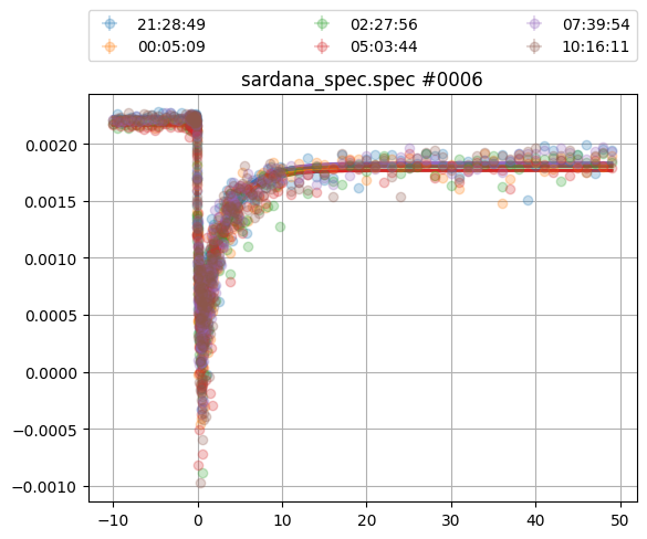
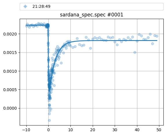
The results does already look very good, but lets access some more information:
plt.figure()
res, parameters, sequence_data = ev.fit_scan_sequence(scan_sequence, mod, pars,
                                                      xgrid=np.r_[-10:50:0.01],
                                                      sequence_type='text',
                                                      show_single=True,
                                                      fit_report=1)
plt.show()
========== Parameter: 21:28:49 ===============

---------- abs_mag: ---------------
          mu:  -1.1282e-01
        tau1:  1.4375e-01
        tau2:  2.7683e+00
           A:  1.8572e-01
           q:  5.1436e+00
       alpha:  1.0000e+00
        sigS:  5.0000e-02
        sigH:  0.0000e+00
          I0:  2.2348e-03
---------------------------------------------------------------------------
TypeError                                 Traceback (most recent call last)
Cell In[31], line 2
      1 plt.figure()
----> 2 res, parameters, sequence_data = ev.fit_scan_sequence(scan_sequence, mod, pars,
      3                                                       xgrid=np.r_[-10:50:0.01],
      4                                                       sequence_type='text',
      5                                                       show_single=True,
      6                                                       fit_report=1)
      7 plt.show()

File ~/checkouts/readthedocs.org/user_builds/pyevaldata/envs/latest/lib/python3.9/site-packages/pyEvalData/evaluation.py:1219, in Evaluation.fit_scan_sequence(self, scan_sequence, mod, pars, ylims, xlims, fig_size, xgrid, yerr, xerr, norm2one, binning, sequence_type, label_text, title_text, ytext, xtext, select, fit_report, show_single, weights, fit_method, offset_t0, plot_separate, grid_on, last_res_as_par, sequence_data, fmt)
   1216 gs = mpl.gridspec.GridSpec(
   1217     2, 1, height_ratios=[1, 3], hspace=0.1)
   1218 ax1 = plt.subplot(gs[0])
-> 1219 markerline, stemlines, baseline = plt.stem(
   1220     x2plot-offsetX, out.residual, markerfmt=' ',
   1221     use_line_collection=True)
   1222 plt.setp(stemlines, 'color',
   1223          plot[0].get_color(), 'linewidth', 2, alpha=0.5)
   1224 plt.setp(baseline, 'color', 'k', 'linewidth', 0)

TypeError: stem() got an unexpected keyword argument 'use_line_collection'
Access fit results#
The results of the fits are given in the res dictionary. Here the keys correspond
again to the elements in the clist:
print(res.keys())
For every counter in the clist we have a nested dictionary with all best values
and errrors for the individual fit parameters. Moreover, we can access some general
parameters as the center of mass (CoM) or integral (int), as well as the
fit objects themselve.
print(res['abs_mag'].keys())
So let’s plot the decay amplitude A for the different parameters in the
scan_sequence:
plt.figure()
plt.errorbar(parameters, res['abs_mag']['A'], yerr=res['abs_mag']['AErr'], fmt='-o')
plt.xlabel('scan time')
plt.ylabel('decay amplitude')
plt.show()
Filters#
# to be done